The Mixed Integer 0-1 Knapsack Problem

by: Brent Austgen, PhD
Dec 13, 2023

Note: Thanks to Shraddha Ghatkar for pointing out an error in my implementation that I have since fixed.

Shortly after publishing my last blog post on the 0-1 knapsack problem, I was privately messaged with a question about using dynamic programming to solve a variant of the standard 0-1 knapsack problem in which some of the binary variables are relaxed to the unit interval. In this post, I address how to modify the dynamic programming approach to solve this variant.

Standard 0-1 Knapsack

Recall the formulation of the standard 0-1 knapsack problem:

$$ \begin{aligned} \max~~ & \sum_{i=0}^{n-1} c_i x_i \\ \text{s.t.}~~ & \sum_{i=0}^{n-1} a_i x_i \le b, \\ & x_i \in \{0, 1\}, \quad i=0,\ldots,n-1. \end{aligned} $$

This problem may be solved via dynamic programming using the value function

$$ \begin{equation*} Z(i, k) = \begin{cases} \max\{Z(i - 1, k), \\ \phantom{\max\{} Z(i - 1, k - a_i) + c_i\}, & k \ge 0, i \ge 0, \\ 0, & k \ge 0, i < 0, \\ -\infty, & k < 0. \end{cases} \end{equation*} $$

The function $Z(i, k)$, a recurrence relation, is the value that may be garnered from discrete items $0$ through $i$ with $k$ space remaining in the knapsack. Note that in my previous post I used $j$ to represent the remaining space. In this post, I use $j$ to index the continuous items and $k$ to represent the remaining space.

Mixed Integer 0-1 Knapsack

To formulate the mixed integer variant, we add new continuous variables $y_j, j=0,\ldots,m-1$ corresponding to $m$ continuous items. Each item $j$ has size $r_j$ and value $t_j$. The formulation for this variant is

$$ \begin{aligned} \max~~ & \sum_{i=0}^{n-1} c_i x_i + \sum_{j=0}^{m-1} t_j y_j \\ \text{s.t.}~~ & \sum_{i=0}^{n-1} a_i x_i + \sum_{j=0}^{m-1} r_j y_j \le b, \\ & x_i \in \{0, 1\}, \quad i=0,\ldots,n-1, \\ & y_j \in [0, 1], \quad j=0,\ldots,m-1. \end{aligned} $$

To solve this variant using dynamic programming, we use a very similar value function:

$$ \begin{equation*} Z(i, k) = \begin{cases} \max\{Z(i - 1, k), \\ \phantom{\max\{} Z(i - 1, k - a_i) + c_i\}, & k \ge 0, i \ge 0, \\ \widehat{Z}(k), & k \ge 0, i < 0, \\ -\infty, & k < 0. \end{cases} \end{equation*} $$

The only difference is the value for the base case $k \ge 0, i < 0$ (i.e., the case in which all discrete items have been considered and the knapsack is not overfilled). In the standard 0-1 knapsack problem, the value is zero in this case. In this variant the value is $\widehat{Z}(k),$ which represents the value that may by garnered from the additional $m$ continuous items if $k$ space remains available in the knapsack. That is, $\widehat{Z}(k)$ is the objective value of a continuous knapsack problem. Of course, George Dantzig proved in 1957 that the continuous knapsack problem may be solved by a greedy heuristic. That heuristic is specifically to put items in the knapsack in decreasing order of $t_j / r_j$ (i.e., in decreasing order of their value-to-size ratio) until it is full. As such, after each combination of discrete items is evaluated via dynamic programming, the continuous items may be considered all at once as a final value-add.

Below, I present a Python implementation of the dynamic programming approach for this problem. The function knapsack_mixed takes as arguments the list of discrete item sizes $\boldsymbol{a},$ the list of continuous item sizes $\boldsymbol{r},$ the knapsack capacity $b,$ the list of discrete item values $\boldsymbol{c},$ and the list of continuous item values $\boldsymbol{t}$.

 1from functools import cache
 2
 3
 4def knapsack_mixed(a, r, b, c, t):
 5
 6    @cache
 7    def Z(i, k):
 8        if i >= 0 and k >= 0:
 9            return max(Z(i - 1, k), Z(i - 1, k - a[i]) + c[i])
10        elif k < 0:
11            return -float('inf')
12        else:
13            Zhat = 0
14            for j in sorted(range(len(r)), key=lambda j: t[j] / r[j], reverse=True):
15                Zhat += t[j] * min(1, k / r[j])
16                k -= r[j] * min(1, k / r[j])
17                if k == 0:
18                    break
19            return Zhat
20
21    def X_and_Y(k):
22        X_opt = [0] * len(a)
23        for i in range(len(a) - 1, -1, -1):
24            X_opt[i] = int(Z(i - 1, k - a[i]) + c[i] > Z(i - 1, k))
25            k -= a[i] * X_opt[i]
26            if k == 0:
27                break
28        Y_opt = [0] * len(r)
29        for j in sorted(range(len(r)), key=lambda j: t[j] / r[j], reverse=True):
30            Y_opt[j] = min(1, k / r[j])
31            k -= r[j] * Y_opt[j]
32            if k == 0:
33                break
34        return X_opt, Y_opt
35
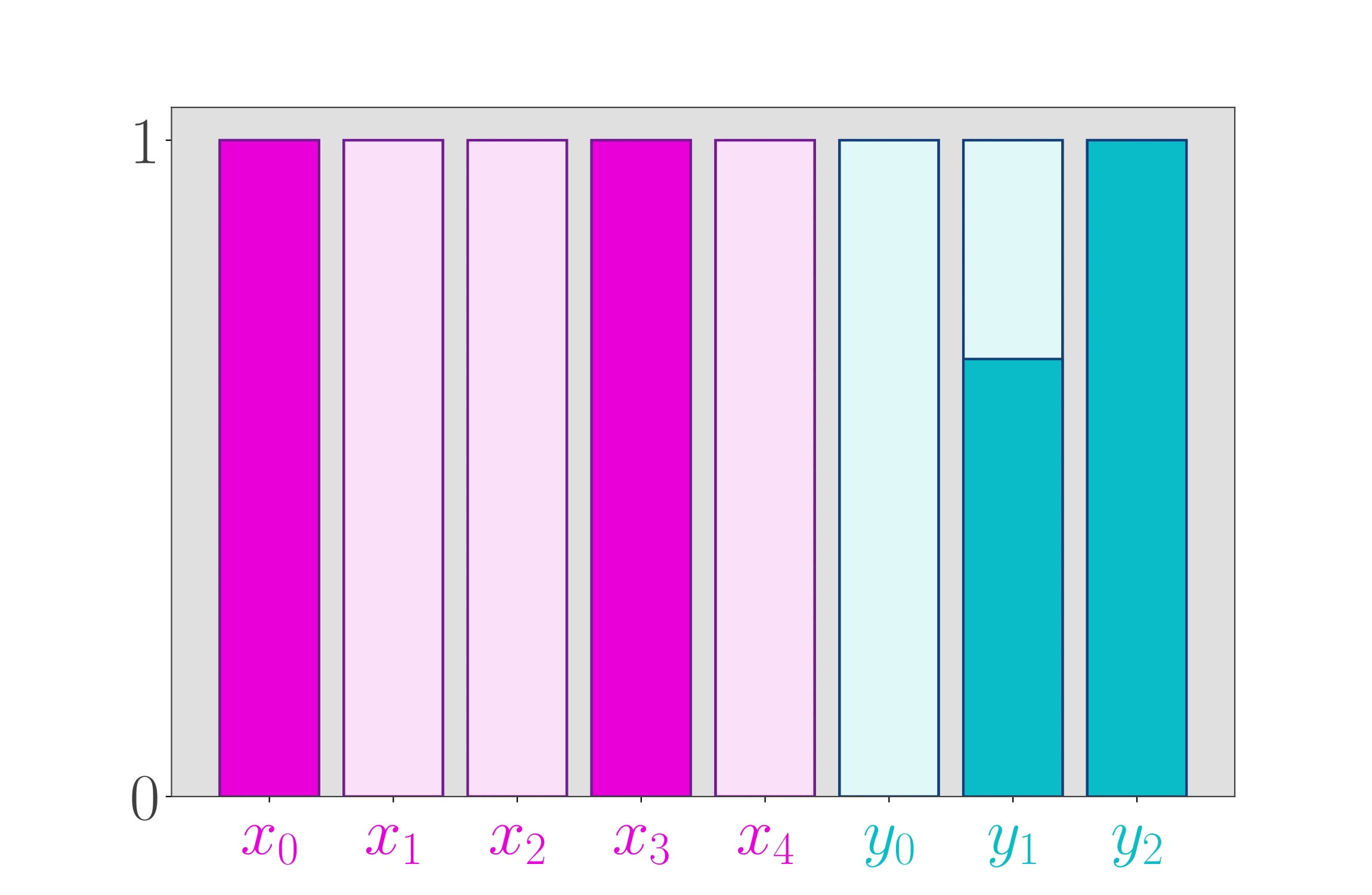
36    return Z(len(a) - 1, b), *X_and_Y(b)

Below, we split the items from the previous post into discrete and continuous sets (not necessarily in the same order). We then run our dynamic programming implementation to find the optimal solution.

 1
 2
 3
 4
 5
 6
 7
 8
 9
10
11
12


### data ###
a = [ 2,  7,  1,  4,  2,  9,  5,  7,  1]
c = [10,  8,  4, 12,  5, 18, 14, 16,  3]
b = 30
r = [ 3,  5,  6,  8, 10,  3]
t = [15,  7,  6, 11, 20,  9]

### dynamic programming ###
print(*knapsack_mixed(a, r, b, c, t))

### print output ###
# 92.0, [0, 0, 1, 1, 1, 0, 1, 1, 1], [1, 0, 0, 0, 0.4, 1]

The solution involves putting 6 of the 9 discrete items into the knapsack. Additionally, two of the continuous items are put in their entirety into the knapsack, and two-fifths of another continuous item is also put into the knapsack.

Invoking the function with r and t as empty lists will produce a solution to a standard 0-1 knapsack problem. Similarly, invoking the function with a and c as empty lists will produce a solution to the continuous knapsack problem (in which the quantity of each item is bounded to $[0, 1]$).