Finally, I reached the end of a rather turbulent academic term and have made the time to look through some COVID-19 data. Better late than never, right? Now in June, it seems the peak of COVID is behind us and almost every state in the U.S. has started to relax COVID-related restrictions. A few states have even lifted restrictions completely.

For my research work, I have recently needed to develop some geographic data processing and visualizing skills. The available tools have really impressed me, so this post is dedicated to showcasing some of them. Since my research is not yet at a stage where I should be sharing results, I figured that COVID should suffice as an interesting and probably more relevant topic. So specifically, this post provides step-by-step instructions on how to produce this spatiotemporal COVID-19 illustration, a sample of which is shown below, using primarily the pandas and plotly Python packages. Note that the full illustration has an interactive time element and may take a moment to fully load, as it is a large file.

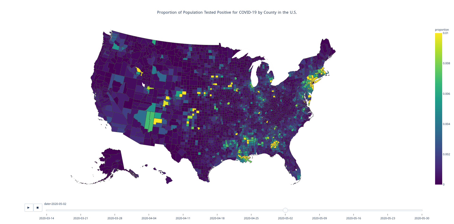
I figure at least few of you all are probably more interested in viewing the illustration than understanding how it was generated. For that reason, let me provide a few disclaimers up front. First, my COVID case numbers were taken from data publicly available from The New York Times. Second, the data has records from as early as January 21, 2020 and has a time resolution of days. My illustration has a time resolution of weeks and shows data only from March 14, 2020 and later. Finally, I artificially clipped the color scale at 0.01 (i.e. 1%). There are indeed quite a few counties with values in excess of that. So while the darkest blue in the image represents exactly 0%, bright yellow is indicative of at least 1% of the county’s population having been infected. In Trousdale County, Tennessee, over 12% of the population has been infected. And if you’re curious, this is why. But had I used 12%, an outlier, as the top of the (linear) color scale, most of the country would have appeared as blue, even at the last time step. Maybe I should have used a logarithmic color scale. Oh well. At the end of the day, there are very many ways to paint the data. I am not trying to induce a panic or play COVID off as nothing, I just wanted to showcase some tools for creating this type of illustration.

So what can you expect from the rest of this article?

• A comprehensive approach to producing the COVID-19 visualization linked above.
• A look at some popular Python tools for handling geographic data.
• Fun facts about county changes from the past decade in the United States.

And what won’t you get?

• Hot takes on COVID-19.
• In-depth analysis of the case data. (But I do encourage you to do some analyis of your own!)

Tools

To get started, I import a few modules to help get the job done. The first group of modules are from the Python standard library. Both urllib and json will be used to retrieve the county border data from the Internet. The second group of modules are some (popular) 3rd-party modules. The pandas has become the standard for processing data tables in Python. As their names suggests, plotly is a plotting package and shapely is a package for processing shapes (i.e. lines, polygons, etc.).

1
2
3
4
5
6
7

import json
from urllib.request import urlopen

import pandas as pd
import plotly.express
import plotly.offline
from shapely.geometry import asShape, mapping

Procuring and Processing the Data

Of course, I did not myself go collect all my own data. I use the geographic county boundary data hosted by the developers of plotly. My COVID-19 data is from the New York Times, and my population data are 2019 estimates provided by the U.S. Census Bureau based on the 2010 census. results. These can all be conveniently downloaded on-the-fly using Python tools.

1
2
3
4
5
6
7

borders_link = 'https://raw.githubusercontent.com'\
               '/plotly/datasets/master/geojson-counties-fips.json'
cases_link = 'https://raw.githubusercontent.com'\
             '/nytimes/covid-19-data/master/us-counties.csv'
populations_link = 'https://www2.census.gov'\
                   '/programs-surveys/popest/datasets/2010-2019/counties'\
                   '/totals/co-est2019-alldata.csv'

First, I download and process the county border data. Remember those fun facts I promised? This data (which ships in GeoJSON format) is a bit old – from 2013 at the latest. How did I come to discover this? The first sign was that my visualization initially did not show the present-day county of Oglala Lakota in South Dakota. After digging, I discovered I was also missing data for the less visible regions of Kusilvak Burough in Alaska and the no longer existing independent city of Bedford in Virginia. So what gives?

• In 2011, officials from the independent city of Bedford, Virginia, in coordination with Bedford County officials pushed papers to transition the city to a town and for it to be reincorporated into the county. These changes went into effect later in 2013. (Hence why I believe the dataset is at least that old.)
• In 2015, the people of Shannon County in South Dakota voted to rename their county to Oglala Lakota. Along with the name change, the FIPS code also changed, and I’ll get to what those are in just a moment.
• Did you know that Alaska does not have counties, but buroughs instead? One of Alaska’s buroughs used to be called Wade Hamption. It was named after Wade Hamption III, an officer of the Confederate States Army and also a slaveholder. In 2015, following a century of controversy, that burough was renamed to Kusilvak, the native name for the mountain range in that region. Again, the FIPS code also changed.

FIPS is an acronym for Federal Information Processing Standards. Each state and territory has an associated 2-digit FIPS code. Moreover, each county has a 3-digit FIPS code. To distinguish two counties from different states that share the same FIPS code, the 5-digit concatenation of state and county FIPS codes is used, and that information is paramount to correctly linking the three datasets together. I could perhaps have found an up-to-date dataset, but I decided to just update this data myself.

First, I modify the FIPS codes for Oglala Lakota County and Kusilvak Burough. Next, I eliminate Bedford City and merge its geography with that of Bedford County using functions and objects from the shapely package. After completing those tasks, I then eliminate records for the United States territories. Finally, I create a df_geo table containing the retained FIPS code. This is used to ensure that data is produced for all U.S. counties (and buroughs!), even those not reporting COVID-19 cases, and only for those counties (and not, for example, for territories). Counties not reporting COVID-19 cases are (naively) assumed to have zero cases.

 1
 2
 3
 4
 5
 6
 7
 8
 9
10
11
12
13
14
15
16
17
18
19
20
21
22
23
24
25
26
27
28
29
30
31
32
33
34

with urlopen(borders_link) as response:
    counties = json.load(response)

for feature in counties['features']:
    props = feature['properties']
    if props['NAME'] == 'Shannon' and props['STATE'] == '46':
        oglala_lakota_county = feature
    if props['NAME'] == 'Wade Hampton' and props['STATE'] == '02':
        kusilvak_burough = feature
    if props['STATE'] + props['COUNTY'] == '51515':
        bedford_city = feature
    if props['STATE'] + props['COUNTY'] == '51019':
        bedford_county = feature

oglala_lakota_county['id'] = '46102'
oglala_lakota_county['properties']['NAME'] = 'Oglala Lakota'
oglala_lakota_county['properties']['COUNTY'] = '102'
oglala_lakota_county['properties']['GEO_ID'] = '0500000US46102'

kusilvak_burough['id'] = '02158'
kusilvak_burough['properties']['NAME'] = 'Kusilvak'
kusilvak_burough['properties']['COUNTY'] = '158'
kusilvak_burough['properties']['GEO_ID'] = '0500000US02158'

counties['features'].remove(bedford_city)
geo_sm = asShape(bedford_city['geometry'])
geo_lg = asShape(bedford_county['geometry'])
bedford_county['geometry'] = mapping(geo_lg.union(geo_sm))

exclude_fips = ['60', '66', '69', '72', '78']
fips = [feature['properties']['STATE'] + feature['properties']['COUNTY']
        for feature in counties['features']
        if feature['properties']['STATE'] not in exclude_fips]
df_geo = pd.DataFrame(data={'fips': fips})

Next, I retrieve and process the population data. Thankfully, this data is highly consistent and requires little effort to use. The biggest hassle I had with this data was determing its encoding standard. There are several features in this dataset, however, I keep only the 5-digit FIPS code (which is constructed from the separate state and county FIPS codes) and the 2019 population estimate.

 1
 2
 3
 4
 5
 6
 7
 8
 9
10
11
12
13
14
15
16
17
18
19

df_pop = pd.read_csv(
    populations_link,
    encoding='ISO-8859-1',
    usecols=[
        'STATE',
        'COUNTY',
        'POPESTIMATE2019'
    ],
    dtype={
        'STATE': 'str',
        'COUNTY': 'str',
        'POPESTIMATE2019': 'int'
    }
)
df_pop['fips'] = df_pop['STATE'] + df_pop['COUNTY']
df_pop.drop(columns=['STATE', 'COUNTY'], axis=1, inplace=True)
df_pop.rename({'POPESTIMATE2019': 'population'}, axis=1, inplace=True)
df_pop = df_geo.merge(df_pop, how='left', on='fips')
df_pop.set_index('fips', inplace=True)

Finally, I work on the COVID data. Each record from this dataset is associated with a 5-digit county FIPS code, a date, and the number of cases and deaths (both cumulative) reported in that county on that date. Our focus is on cases, so I drop the deaths data in the retrieval process. There is some superfluous state-level aggregate data for which the FIPS code is missing. That is fine though, as it makes it easy for us to ignore – we simply drop all records for which the FIPS code is undefined.

1
2
3
4
5
6
7
8
9

df_numbers = pd.read_csv(
    cases_link,
    dtype={
        'date': 'str',
        'fips': 'str',
        'cases': 'int'
    }
)
df_numbers.dropna(subset=['fips'], inplace=True)

For this application, there are a few problems with the case data.

1. Some counties have not reported at all.
2. Most counties have reported, but on irregular and disjoint schedules. That is, not all counties are reporting on a daily basis.
3. Data incoherence. There are a few instances of the number of cases falling from one day to the next. These are infrequent, so I chalk this up to data entry error but address it nonetheless.

To remedy, I pivot the table to have a row for every county and a column for every day. Due to the issues described above, this creates a table with many missing values. I replace all missing values with zeros, then apply a cumulative maximum function to ensure that cumulative cases are guaranteed to be non-decreasing in time. For each county, I then divide the case count at each time step by the population of the county to obtain proportion values. Finally, I melt the table. A melt is the opposite of a pivot, so I am left with a table that is similar in shape to that of the original – one column for FIPS code, one for date, and one of the proportions. However, the data is much cleaner after this process – I now have coherent data for every county and for every date from January 21, 2020 to present.

 1
 2
 3
 4
 5
 6
 7
 8
 9
10
11
12
13
14
15

df_cases = df_numbers.pivot(index='fips',
                            columns='date',
                            values='cases')\
                     .merge(df_geo,
                            how='right',
                            left_index=True,
                            right_on='fips')\
                     .set_index('fips')\
                     .fillna(0)\
                     .cummax(axis=1)\
                     .div(df_pop['population'], axis=0)\
                     .reset_index()\
                     .melt(id_vars='fips',
                           var_name='date',
                           value_name='proportion')

Creating the Illustration

With the data now in a suitable format, all that’s left is to plot it. This data is large. In an effort to reduce the size, I create a filter that allows me to get just the values from every Sunday beginning on March 14, 2020. I choose not to show data from before that date due to disparity of scale. To plot the data, I use the choropleth function provided in plotly.express and pass it my filtered table. The county borders are all associated with a FIPS code. To match my data to the geographic regions, I tell the function to use the 'fips' column of my data. The color of each county is determined by the scale (which I define as the interval from 0% to 1%), and by the data in the 'proportion' column of my table. To create an animation, I tell the function to use the 'date' column to distinguish between frames.

 1
 2
 3
 4
 5
 6
 7
 8
 9
10
11
12
13
14
15
16
17
18
19
20

dates = df_cases['date'].sort_values().unique().tolist()
mask = df_cases['date'].isin(dates[dates.index('2020-03-14')::7])
lower_bound = 0.0 / 100
upper_bound = 1.0 / 100
title = 'Proportion of Population Tested Positive '\
        'for COVID-19 by County in the U.S.'

fig = plotly.express.choropleth(
    df_cases.loc[mask],
    geojson=counties,
    locations='fips',
    animation_frame='date',
    color='proportion',
    color_continuous_scale='viridis',
    range_color=(lower_bound, upper_bound),
    scope='usa',
    title=title
)
fig.update_layout(title_x=0.5)
fig.update_layout(margin={"r": 0, "l": 0, "b": 0})

Do not be surprised if this code does not complete quickly, it might take a minute or two. But then that’s it. Nothing left to do except perhaps save the illustration to an HTML file, just as I did to host it on my website. That can be accomplished with the following one line.

1

plotly.offline.plot(fig, filename='covid.html')

Like always, feel free to let me know your thoughts in the comments below. Ideas, questions, and comments are all welcome.