This past week saw the debut of PEP572 in the release of Python 3.8.0. A PEP is a Python Enhancement Proposal, a document that describes a feature and requests its incorporation into the Python language. Now PEP572 in particular was about as controversial as they come, so much so that it caused Guido von Rossum, the original author of Python, to step down from his role as Benevolent Dictator for Life and form a committee to replace him. Yikes!

What is PEP572?

So why the controversy? Well, the aim of this PEP was to introduce the walrus operator := to perform assignments in ways that were previously not possible, e.g., inside a tuple declaration or in a while-loop condition. Oh, and in case you were wondering, the walrus operator is named so for its resemblance to the eyes and tusks of a walrus. You can see it if you squint. Anyhow, not such a radical idea, is it? Well, there are those with this or that argument against it like “it detracts from readability” or “it is only useful as a shim to poorly implemented libraries” or “it will not be backward compatible with older versions of Python 3.x”. Despite the merits of these arguments, PEP572 was accepted and implemented for better or for worse.

I’ve been tracking PEP572 for a while. Not since its inception, but a while. And now that it’s here in the official Python 3.8 release, I figured it could use a little promotion. Here’s a taste.

1

z = (x := 'foo', y := 'bar', 'baz')

This example is intuitive, but not very useful in practice. It is inferior to a more readable equivalent that ignores a value using the conventional underscore.

1

z = (x, y, _) = ('foo', 'bar', 'baz')

These snippets both result in the tuple ('foo', 'bar', 'baz') being assigned to z and the strings 'foo' and 'bar' being assigned to x and y, respectively.

Newton’s Method

In my opinion, the best use of the walrus operator is to reduce code size in initialize-iterate-reassign patterns. In this section, I illustrate that benefit in the context of an implementation of Newton’s method.

Newton’s method is an iterative numerical method for finding roots of functions. A root of a function $f(x)$ is a constant $a$ that satisfies $f(a) = 0$ . That is, plug $a$ into the function, and $0$ comes out.

Roots are sometimes trivial to find. For example, suppose $f(x) = x - 1$ . By inspection, we find the root by setting $x - 1 = 0$ and solving for $x$ to get $1$ . Newton’s method really shines when the roots are difficult to find analytically or when multiple roots exist.

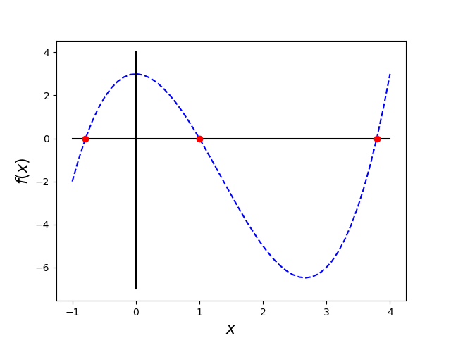
For the rest of this article, let’s consider the 3rd-order polynomial function $f(x) = x^3 - 4x^2 + 3$ with derivative $f^\prime(x) = 3x^2 - 8x$ . Here is its graph. In Python, here is how we define this function and its derivative. Later, these functions will be passed as objects to our implementations of Newton’s method. Remember that virtually everything in Python is an object, even a function!

1
2
3
4
5

def f(x):
    return x ** 3 - 4 * x ** 2 + 3

def fprime(x):
    return 3 * x ** 2 - 8 * x

A bit of quick guess-and-check or a look at the graph tells us the value $1$ is a root of this function. But a 3rd-order polynomial can have as many as 3 roots! As we can see, this one has exactly 3 roots and the remaining two are not nearly as easy to calculate. So we employ a simple form of Newton’s method that is based on the following recurrence relation:

Below is a code implementation of Newton’s method that does not use the walrus operator.

1
2
3
4
5
6
7

def old_newtons_method(f, fprime, x_0, tol=1e-6):
    x_curr = x_0
    x_next = x_curr - f(x_curr) / fprime(x_curr)
    while abs(x_curr - x_next) > tol:
        x_curr = x_next
        x_next = x_curr - f(x_curr) / fprime(x_curr)
    return x_curr

This code is functionally correct. It is, however, a little clunky. The logic that is used to initialize x_next is repeated inside in the for-loop to iterative update x_next.

To reduce code size, we might try a slightly different implementation that still does not include the walrus operator.

1
2
3
4
5

def bad_newtons_method(f, fprime, x_0, tol=1e-6):
    x_curr = x_0
    while abs(f(x_curr) / fprime(x_curr)) > tol:
        x_curr = x_curr - f(x_curr) / fprime(x_curr)
    return x_curr

The Walrus Operator

Ask and you shall receive.

1
2
3
4
5

def new_newtons_method(f, fprime, x_0, tol=1e-6):
    x_curr = x_0
    while abs(delta_x := f(x_curr) / fprime(x_curr)) > tol:
        x_curr = x_curr - delta_x
    return x_curr

Ah, beautiful! Notice the walrus operator in the middle of the while condition. Not only does this code perform just as well as the first implementation, it is more compactly written than either of the previous two examples. And yes, this code is also functionally correct.

Now, let’s use what we’ve built!

1
2
3
4
5
6

roots = [
    new_newtons_method(f, fprime, -1)
    new_newtons_method(f, fprime, 2)
    new_newtons_method(f, fprime, 4)
]
print(roots)

Using the carefully handpicked initial guesses of $-1, 2,$ and $4$, we ascertain that the roots are roughly $-0.791, 1.000,$ , and $3.791$. If we look back to our graph of this function, we can visually verify these roots. Neat!

Like what you learned? Did I make a mistake? Let me know in the comments! Happy root-finding!