In the realm of algorithms and graph theory, two of the most famous optimization problems are Max-Flow and Min-Cut. The Max-Flow problem involves finding the optimal flow in a network, much like water through pipes or traffic on roads. The Min-Cut problem is about finding the minimum capacity of edges that, if removed from a network, would disconnect its source from its sink, effectively reducing the flow between them to zero. Both of these problems are formulatable as a linear program (LP) and, in fact, are intricately linked by a strong dual relationship. In this post, we introduce the Max-Flow problem and its rudimentary LP formulation. We then motivate an equivalent but more consistent formulation based on an augmented graph. Using a matrix/vector representation, we present the primal and dual LPs and walk through the interpretation of the dual LP as the Min-Cut problem.

This post is part 1 of a 2-part series. This part focuses on the linear programming formulations of the Max-Flow problem, matrix/vector representations of the problem based on the graph’s node/edge adjacency matrix, and the dual relationship between Max-Flow and Min-Cut. In the second part, we develop implementations of these two graph optimization problems in gurobipy and visualize the solutions by leveraging both primal and dual variable values.

Max-Flow Primal LP

The Max-Flow problem is defined on a directed graph $G = (V, E)$ where $V$ and $E$, repsectively, denote the sets of vertices and edges. The term “directed” simply means that each edge is like a one-way street – flow is unidirectional. The goal of the Max-Flow problem is to maximize the flow from the source node $s$ to the sink node $t$ subject to limits on the flow allowed across each edge in the graph.

To formulate the problem, let ${V_i^+ = \{j : (j, i) \in E\}},$ and ${V_i^- = \{j : (i, j) \in E\}}.$ The set $V_i^+$ represents the vertices neighboring $i$ via entering edges and $V_i^-$ the set neighboring $i$ via exiting edges. For $(i, j) \in E$, let $x_{ij} \in \mathbb{R}_+$ be a variable representing the flow on edge $(i, j)$, and let $c_{ij}$ be its upper bound. Then the Max-Flow problem may be formulated as

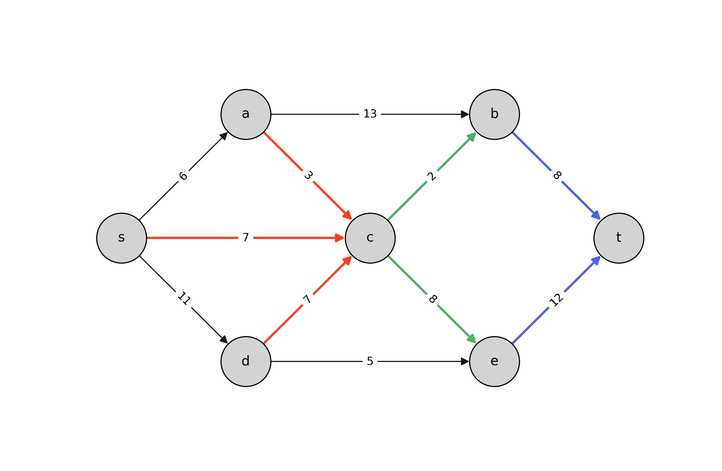
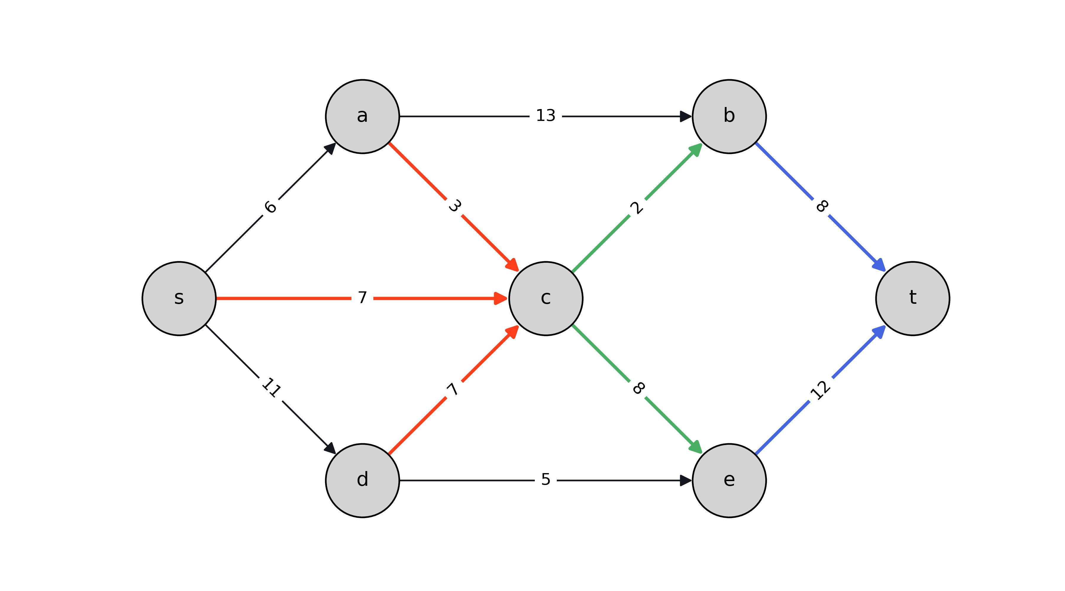
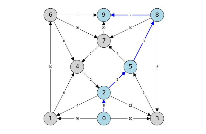
In the image below, we link the formulation to a specific graph.Edges entering the sink node are colored blue to match the corresponding sum in the objective function of the formulation. At node $c$, entering edges are colored red and leaving edges are colored green to illustrate the flow balance constraints at that node. In this formulation, the objective is to maximize the sum of flows on all the edges entering the target vertex. For the sake of simplicity, we suppose that $c_{ij} > 0$ for all $(i, j) \in E$ and that there exists at least one path from $s$ to $t$ such that the solution is guaranteed to be non-trivial (i.e., $z_p^* > 0$). Flow balance is imposed at all vertices except at the sink $t$ where there is ideally a net surplus and at the sink $s$ where there is a corresponding deficit. The flow on each edge is required to be between zero the edge’s capacity.

Intuitively, the total flow entering $t$ ought to be equal to the flow exiting $s$. Indeed, this condition is guaranteed by the flow balance constraints. In summing over those constraints, most flow variables appear exactly once with a positive sign and once with a negative sign. The exceptions are the variables for flows entering $t$ which appear only once with a positive sign and those exiting $s$ which appear only once with a negative sign. Ergo,

Though this condition is superfluous, it is the foundation of a convenient reformulation. Defining a new variable

we observe that

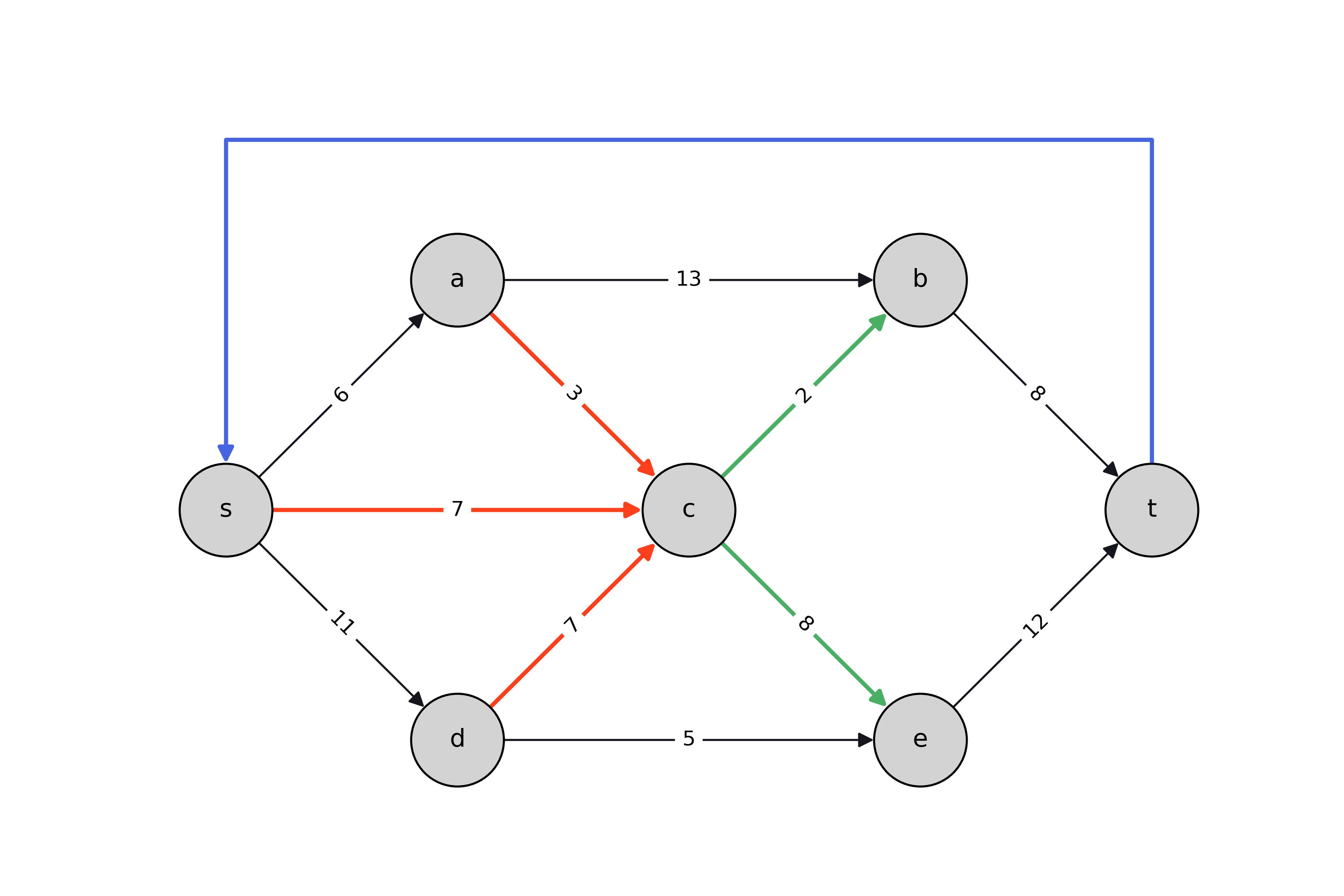
The reformulation is achieved by considering the graph ${\hat{G} = (V, \hat{E})}$ with augmented edge set ${\hat{E} = E \cup \{(t, s)\}}.$ Incorporating such an edge (with unlimited capacity) allows all of the flow entering $t$ to recirculate back to $s$ in a cycle thus making flow balance applicable at every node including $s$ and $t$. Letting $\hat{V}_i^+ = \{j : (j, i) \in \hat{E}\},$ and $\hat{V}_i^- = \{j : (i, j) \in \hat{E}\},$ the reformulated problem is

Below, we illustrate this Max-Flow reformulation. Added edge $(t, s)$ is colored blue to match the corresponding variable objective function. Flow balance at $c$ is illustrated as it was before.

To form the dual of this problem, we rewrite it compactly using matrix and vector quantities and distinguishing between quantities pertaining to the original graph $G$ and added edge $(t, s)$:

Here, $A$ denotes the node/edge adjacency matrix for the original graph $G$. The rows of $A$ are indexed in $V$ and the columns in $E$. The column of $A$ corresponding to edge $(i, j)$ has a $-1$ in the row corresponding to node $i$ and a $1$ in the row corresponding to row $j$. The vector $\boldsymbol{a}_{ts}$ denotes a similar incidence vector for edge $(t, s)$.

Max-Flow Dual LP

Following the simple rules for forming the dual LP, we find the dual of the Max-Flow problem is

Recall the structure of $A$. The column corresponding to edge $(i, j)$ has $1$ in the $j^\text{th}$ position, $-1$ in the $i^\text{th}$ position, and $0$ elsewhere. Likewise, $\boldsymbol{a}_{ts}$ has $1$ in the $s^\text{th}$ position, $-1$ in the $t^\text{th}$ position, and $0$ elsewhere. Incorporating this information, an equivalent formulation of the dual LP is

Dual LP Interpretation as Min-Cut

From complementary slackness, we know that if $x_{ts}^* > 0$, then ${z_s^* - z_t^* = 1}$. It is clear from the problem structure that for each $(i, j) \in E$ the values of $z_i$ and $z_j$ are only important to the extent of their difference $z_i - z_j$. As such, we are free to fix any one $z_i$ to a constant value. Without loss of generality, let us fix $z_t = 0$. Then, again supposing the instance is non-trivial, complementary slackness requires $z_s = 1$ for the dual solution to be optimal.

Next, let $(\boldsymbol{y}^\prime, \boldsymbol{z}^\prime)$ be a feasible dual solution. If ${y_{ij}^\prime > z_i^\prime - z_j^\prime}$ and $y_{ij}^\prime > 0$, then $(\boldsymbol{y}^\prime, \boldsymbol{z}^\prime)$ is suboptimal. To see this, let $\boldsymbol{y}^{\prime\prime}$ be such that ${y_{ij}^{\prime\prime} = \max\{z_i^\prime - z_j^\prime, 0\}}.$ Then, because $c_{ij} > 0$ for all $(i, j) \in E$, the solution $(\boldsymbol{y}^{\prime\prime}, \boldsymbol{z}^\prime)$ is strictly better than $(\boldsymbol{y}^\prime, \boldsymbol{z}^\prime)$. That is, given our suppositions that ensure a non-trivial optimal solution in the primal LP, an optimal solution to the dual LP must satisfy ${y_{ij}^* = \max\{z_i^* - z_j^*, 0\}}.$

With this in mind, it is easy to show that an optimal dual solution must also satisfy $\boldsymbol{0} \le \boldsymbol{z}^* \le \boldsymbol{1}$. Again consider feasible solution $(\boldsymbol{y}^\prime, \boldsymbol{z}^\prime)$. To see this, let $(\boldsymbol{y}^{\prime\prime}, \boldsymbol{z}^{\prime\prime})$ be such that ${z_i^{\prime\prime} = \min\{\max\{z_i^\prime, 0\}, 1\}}$ for all $i \in N$ and ${y_{ij}^{\prime\prime} = \max\{z_i^{\prime\prime} - z_j^{\prime\prime}, 0\}}$ for all $(i, j) \in E$. That is, let $\boldsymbol{z}^{\prime\prime}$ be $\boldsymbol{z}^\prime$ clipped to $[0, 1]$ and let $\boldsymbol{y}^{\prime\prime}$ satisfy the criteria for optimality. For each edge $(i, j)$, there are three cases to consider:

1. If $z_i^\prime \le z_j^\prime$, then $z_i^{\prime\prime} \le z_j^{\prime\prime}$ so $y_{ij}^{\prime\prime} = 0 \le y_{ij}^\prime$.
2. If $z_i^\prime > z_j^\prime$ and $z_i^\prime \!\in\! [0, 1]$ and $z_j^\prime \!\in\! [0, 1]$, then $z_i^{\prime\prime} - z_j^{\prime\prime} \!=\! z_i^\prime - z_j^\prime$ so $y_{ij}^{\prime\prime} \le y_{ij}^\prime$.
3. If $z_i^\prime > z_j^\prime$ and either $z_i^\prime \!\not\in\! [0, 1]$ or $z_j^\prime \!\not\in\! [0, 1]$, then $z_i^{\prime\prime}\!-\!z_j^{\prime\prime} \!<\! z_i^\prime\!-\!z_j^\prime$ so $y_{ij}^{\prime\prime} < y_{ij}^\prime$.

If ${z_i^\prime \not\in [0, 1]}$ for at least one $i \in N$, then case (3) is applicable for at least one edge, so $\boldsymbol{y}^{\prime\prime} < \boldsymbol{y}^\prime$ and $\boldsymbol{c}^\top \boldsymbol{y}^{\prime\prime} \le \boldsymbol{c}^\top \boldsymbol{y}^\prime$. Ergo, an optimal solution to the dual LP must also satisfy $0 \le z_i^* \le 1$. As such, $z_i^* - z_j^* \le 1$ for every $(i, j) \in E$ so ${0 \le y_{ij}^* = \max\{z_i^* - z_j^*, 0\} \le 1}$ as well.

Finally, note that the constraint coefficients in this problem form a totally unimodular matrix. As such, all extreme point solutions are integral. Since, as we discussed, all optimal solutions are confined to $[0, 1]^{|V| + |E|}$, all the extreme point solutions are not just integral solutions but 0/1 solutions. Since every LP has an extreme point solution that is optimal, there exists at least one optimal 0/1 solution. Of course, it is possible for two or more 0/1 solutions to exist, and in that case there also exist infinitely many non-integral solutions in their convex hull.

The crux of all this analysis is that there exists an integer programming (IP) restriction of the Max-Flow dual LP that yields the same $z_d^*$. Its formulation is

In this IP, $\boldsymbol{z}$ encodes a vertex bipartition: $i \in A$ if $z_i = 1$ or $i \in B$ if $z_i = 0$. Because $z_s = 1$ and $z_t = 0$, the only feasible partitions are those that separate $s$ from $t$, and in fact all such partitions are feasible. Similarly, $\boldsymbol{y}$ encodes the minimal directed cut that separates $A$ from $B$ and thus separates $s$ from $t$: $(i, j)$ in the cut if $y_{ij} = 1$ or not in the cut if $y_{ij} = 0$. To see that the cut indeed separates $s$ from $t$, consider that for every path $P$ from $s$ to $t$, the constraints require that That is, the constraints require that at least one edge in every path from $s$ to $t$ participates in the cut. An example $s$-$t$ cut is shown below. In the image, nodes belonging to sets $A$ and $B$ are, respectively, colored green and red. The minimal cut separating $A$ from $B$ is represented by the dotted edges.

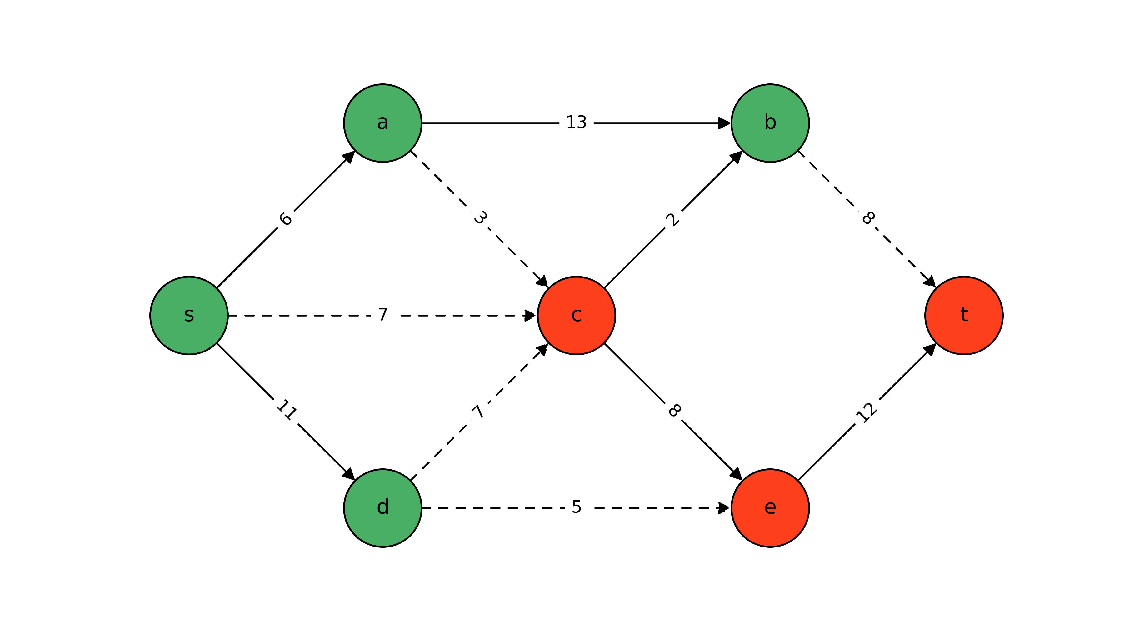
As a closing thought, recall that though the Min-Cut IP formulation in this section is a restriction of the Max-Flow’s dual LP, its objective value is the same. Therefore, by strong duality, the maximum $s$-$t$ flow in a graph is equal to the value of the minimum $s$-$t$ cut (i.e., $z_p^* = z_d^*$). This is in contrast to the weak duality often exhibited by other discrete optimization problems defined on graphs on otherwise. For example, the number of edges in a maximum matching is only sure to be less than or equal to the number of vertices in a minimum edge cover. The strong duality of the continuous Max-Flow problem and discrete Min-Cut problem is remarkable.