As the INFORMS 2023 Annual Meeting comes to an end this week in Phoenix, I thought I should show how to use the somewhat new gurobipy-pandas package that facilitates building models in gurobipy using pandas objects and moreover compare the code to the standard gurobipy-only implementation. I came to learn of this package through a presentation by Robert Luce at Gurobi and subsequent conversations with Robert and contributor Irv Lustig at Princeton Consultants.

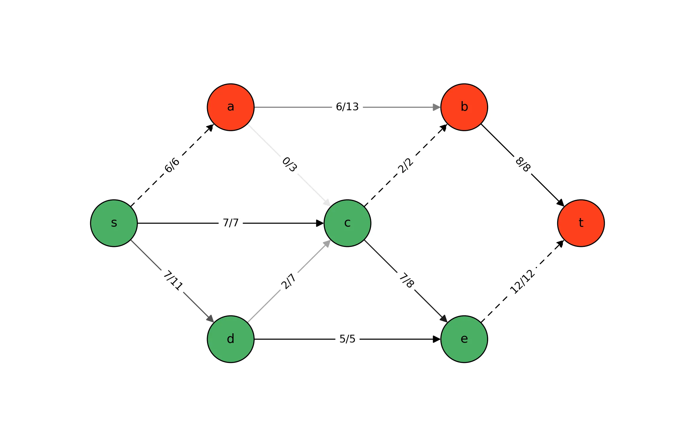
If you’re tired of me posting about the Max-Flow LP model, I have bad news. In this post, we again leverage the Max-Flow optimization model as an example. In this previous post we motivate the following linear programming formulation:

Consider first the following implementation of the Max-Flow LP without pandas:

 1
 2
 3
 4
 5
 6
 7
 8
 9
10
11
12
13
14
15
16
17
18
19
20
21
22
23
24
25
26
27
28
29

from collections import defaultdict
from itertools import chain

import gurobipy as grb


c = {('a', 'b'): 13, ('c', 'b'):  2, ('b', 't'):  8,
     ('a', 'c'):  3, ('c', 'e'):  8, ('d', 'c'):  7,
     ('d', 'e'):  5, ('e', 't'): 12, ('s', 'a'):  6,
     ('s', 'c'):  7, ('s', 'd'): 11}
V = sorted(set(chain.from_iterable(c.index)))
E = list(c)
E_hat = E + [('t', 's')]
Vp_hat = defaultdict(set)
Vm_hat = defaultdict(set)
for (i, j) in E_hat:
    Vp_hat[j].add(i)
    Vm_hat[i].add(j)

maxflow = grb.Model()
x = maxflow.addVars(E_hat)
con_z = maxflow.addConstrs(
    (sum(x[j, i] for j in Vp_hat[i])
     - sum(x[i, j] for j in Vm_hat[i]) == 0)
    for i in V
)
con_y = maxflow.addConstrs(x[i, j] <= c[i, j] for (i, j) in E)
maxflow.setObjective(x['t', 's'], grb.GRB.MAXIMIZE)
maxflow.optimize()

Perhaps the trickiest part of the implementation is defining $\hat{V}_i^+$ and $\hat{V}\_i^-$ and then using those sets to implement the flow balance constraints via comprehensions in lines 24-25 above. Not that this is particularly burdensome for this example, the beauty of gurobipy-pandas (and pandas more generally) is that such comprehensions may be replaced by invoking Series.groupby as in the script below.

 1
 2
 3
 4
 5
 6
 7
 8
 9
10
11
12
13
14
15
16
17
18
19
20
21
22
23
24
25
26
27

from itertools import chain

import gurobipy as grb
import gurobipy_pandas as gppd
import numpy as np
import pandas as pd


c = {('a', 'b'): 13, ('c', 'b'):  2, ('b', 't'):  8,
     ('a', 'c'):  3, ('c', 'e'):  8, ('d', 'c'):  7,
     ('d', 'e'):  5, ('e', 't'): 12, ('s', 'a'):  6,
     ('s', 'c'):  7, ('s', 'd'): 11}
c = pd.Series(c)
c.index.names = ['i', 'j']
c.loc['t', 's'] = None
V = sorted(set(chain.from_iterable(c.index)))

maxflow = grb.Model()
x = gppd.add_vars(maxflow, c, name='x', ub=c.fillna(np.inf),
                  vtype=grb.GRB.CONTINUOUS)
con_z = gppd.add_constrs(maxflow,
                         x.groupby('i').sum().reindex(V).fillna(0),
                         grb.GRB.EQUAL,
                         x.groupby('j').sum().reindex(V).fillna(0),
                         name='con_z')
maxflow.setObjective(x.loc['t', 's'], sense=grb.GRB.MAXIMIZE)
maxflow.optimize()

If every node were to have at least one incoming and outgoing edge, then there would be no need for $V$. Though this occurs in the example we present, it is not generally guaranteed. For the sake of generality, we define the set $V$ so that we may use it for reindexing to ensure the sum of $x_{ij}$ is defined for every node, if even as zero. In this implementation, we enforce $x_{ij} \le c_{ij}$ in the variable declaration unlike how we defined the constraint explicitly in the first implementation.

To avoid having pandas as a dependency for gurobipy, the developers elected to make gurobipy-pandas a separate optional package. As a consequence, the creation of pandas-compatible variables and constraints is achieved by invoking functions of the gurobipy_pandas module rather than by the familiar object methods model.addVar, model.addConstr, and the like.

In short, the main advantages of using gurobipy-pandas and not just gurobipy are (i) that it facilitates a data-first (vs. model-first) approach, (ii), that it allows data to be loaded easily from tabular data files, and (iii) that slicing and groupby/aggregating data in pandas.Series is computationally very efficient.

Which of these two implementations do you prefer? Do you see yourself using gurobipy-pandas in the future? (Are you already!?) Let me know in the comments!