In a previous post, we discussed the strong dual relationship between the Max-Flow and Min-Cut optimization problems, and presented matrix/vector formulations of those problems. In this post, we show how to implement each problem as a linear program (LP) using gurobipy, and then visualize the primal and dual variable values using networkx and matplotlib. As an aside, note that linear programming is generally not the best tool for solving these problems, as there exist specialized algorithms like the Ford-Fulkerson algorithm or Dinic’s algorithm. The purpose of solving these problems as LPs is to demonstrate the extraction of dual variable values in gurobipy and to highlight these problems’ primal-dual relationships.

This post is part 2 of a 2-part series. This part focuses on LP implementations of the Max-Flow and Min-Cut optimization problems in gurobipy, and visualizations of the primal and dual variable values for solved instances. In the first part, we walk through the strong dual relationship between these two problems.

The code from this post is available for download as a Jupyter notebook.

Setup

For this demonstration, we need tools from just a handful of packages.

1
2
3
4
5
6

from collections import defaultdict

import gurobipy as grb
import matplotlib.pyplot as plt
import matplotlib.cm as cm
import networkx as nx

Next, we define the graph parameters and instantiate a networkx.DiGraph for later use.

 1
 2
 3
 4
 5
 6
 7
 8
 9
10
11
12
13
14
15
16

pos = {'s': (0, 1), 'a': (1, 2), 'b': (3, 2), 'c': (2, 1),
       'd': (1, 0), 'e': (3, 0), 't': (4, 1)}
c = {('a', 'b'): 13, ('c', 'b'):  2, ('b', 't'):  8,
     ('a', 'c'):  3, ('c', 'e'):  8, ('d', 'c'):  7,
     ('d', 'e'):  5, ('e', 't'): 12, ('s', 'a'):  6,
     ('s', 'c'):  7, ('s', 'd'): 11}
V = list(pos)
E = list(c)
E_hat = E + [('t', 's')]
Vp_hat = defaultdict(set)
Vm_hat = defaultdict(set)
for (i, j) in E_hat:
    Vp_hat[j].add(i)
    Vm_hat[i].add(j)
graph = nx.DiGraph()
graph.add_edges_from(E)

Linear Programming Formulations

Recall from part 1 that the Max-Flow problem is defined on a directed graph ${G = (V, E)}$ with source node $s$ and sink node $t$. In an equivalent reformulation, the problem is defined on an augmented graph $\hat{G} = (V, \hat{E})$ where $\hat{E} = E \cup \{(t, s)\}.$ The added uncapacitated edge $(t, s)$ completes a cycle that allows the maximum flow to recirculate from $t$ to $s$. Each variable $x_{ij}$ represents the flow on edge $(i, j)$. In the flow balance constraints, ${\hat{V}_i^+ = \{j : (j, i) \in \hat{E}\}}$ and ${\hat{V}_i^- = \{j : (i, j) \in \hat{E}\}}.$ Additionally, $c_{ij}$ denotes the flow capacity of edge $(i, j)$. For the sake of simplicity, we suppose $G$ has at least one path from $s$ to $t$ and that $c_{ij} > 0$ for all $(i, j) \in E$ as the conditions guarantee a non-trivial solution (i.e., $z_p^* > 0$). Using this notation, we presented the following LP formulation of Max-Flow:

Its dual, an LP relaxation of the Min-Cut integer program, is

Linear Programming Implementations

In our code, most of the names are straightforward. Two names that warrant clarification are Vp_hat[i] (“p” for plus) which represents $\hat{V}_i^+$ and Vm_hat[i] (“m” for minus) which represents $\hat{V}_i^-.$ With the parameters already established, only a few lines of code are needed to implement and solve this formulation.

 1
 2
 3
 4
 5
 6
 7
 8
 9
10

maxflow = grb.Model()
x = maxflow.addVars(E_hat)
con_z = maxflow.addConstrs(
    (sum(x[j, i] for j in Vp_hat[i])
     - sum(x[i, j] for j in Vm_hat[i]) == 0)
    for i in V
)
con_y = maxflow.addConstrs(x[i, j] <= c[i, j] for (i, j) in E)
maxflow.setObjective(x['t', 's'], grb.GRB.MAXIMIZE)
maxflow.optimize()

In part 1 we made two observations about the dual LP:

1. Complementary slackness requires that $z_s^* - z_t^* \ge 1$ be binding if $x_{ts}^* > 0$.
2. Given that only differences of the $z_i$ variables are present in the constraints, we are free to fix a single $z_i$ to a constant value.

Since our parameterization of the instance guarantees $x_{ts}^* > 0$ , rather than implement $z_s - z_t \ge 1$ we fix $z_t = 0$ and $z_s = 1$. Our implementation of the LP relaxation of Min-Cut is given below.

 1
 2
 3
 4
 5
 6
 7
 8
 9
10
11

mincut = grb.Model()
y = mincut.addVars(E)
z = mincut.addVars(V, lb=-grb.GRB.INFINITY, ub=grb.GRB.INFINITY)
con_x = mincut.addConstrs(
    y[i, j] >= z[i] - z[j]
    for (i, j) in E
)
z['s'].lb = z['s'].ub = 1
z['t'].lb = z['t'].ub = 0
mincut.setObjective(sum(c[i, j] * y[i, j] for (i, j) in E), grb.GRB.MINIMIZE)
mincut.optimize()

Visualization via Max-Flow

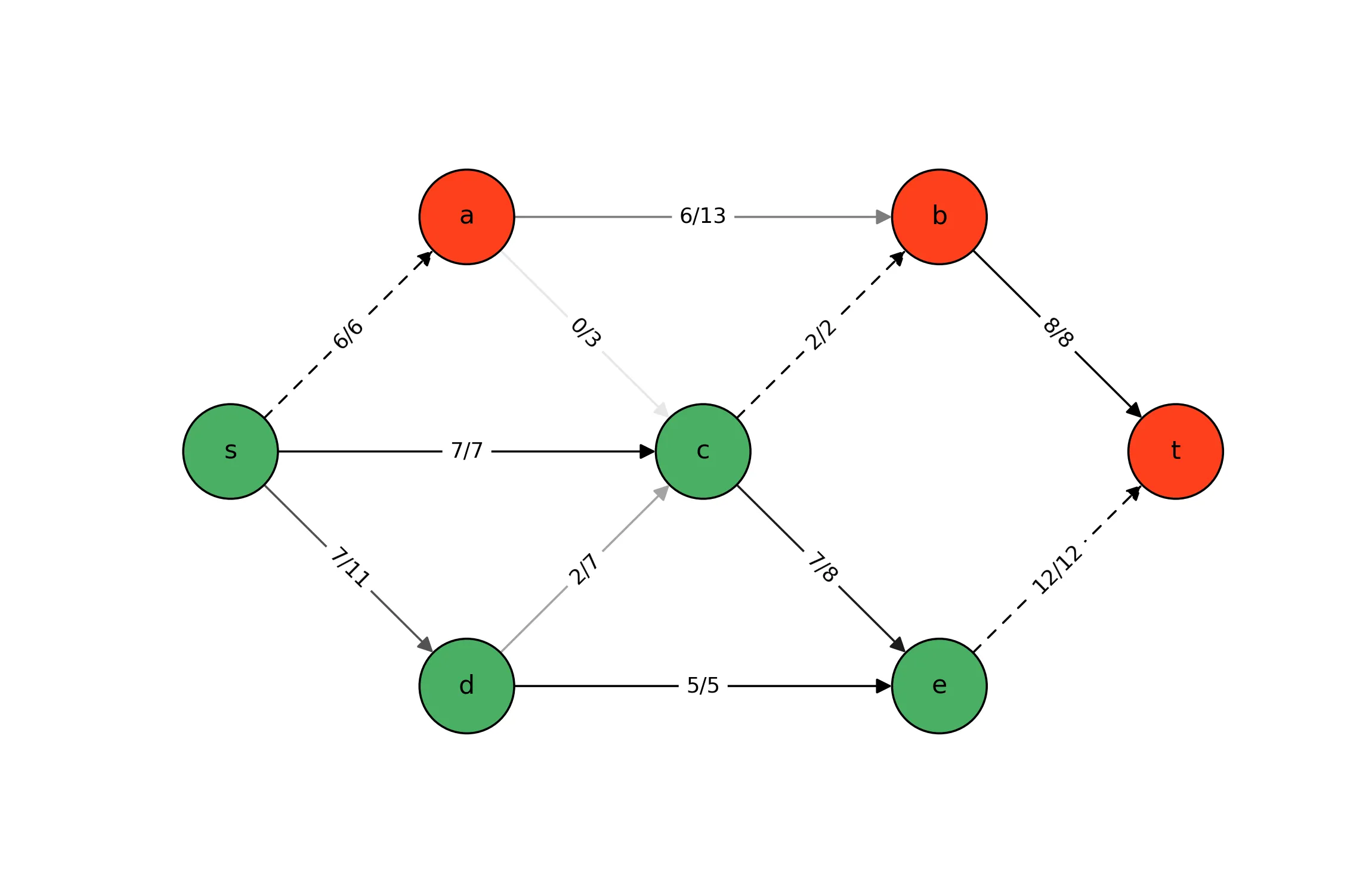
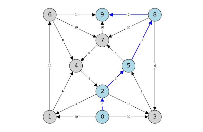
We conclude by visualizing the optimal solutions to these problems that were identified by the Gurobi solver. Each visualization shows both the Max-Flow and Min-Cut solutions. To show the Max-Flow solution, we draw a label on each edge indicating the flow and the capacity. Moreover, we shade the edge to reflect its usage relative to its capacity (light for low usage and dark for high usage). To show the Min-Cut solution, we color the nodes to reflect their bipartitioning (green if in the same group as the source node and red if in the same group as the sink node). Additionally, edges that participate in the cut are drawn with dashed lines.

When using gurobipy, a variable’s value in the current solution is stored as a float to the X attribute. A constraint’s shadow price (i.e., dual variable value) is stored as a float to the Pi attribute of the constraint. After we solve the primal problem, we thus retrieve the Max-Flow solution values via x[i].X and the Min-Cut solution values as con_y[i, j].Pi and con_z[i].Pi. The code for illustrating the solution and the illustration itself are both shown below.

 1
 2
 3
 4
 5
 6
 7
 8
 9
10
11
12
13
14
15
16
17
18
19
20
21
22
23
24
25
26

fig, ax = plt.subplots(figsize=(9, 5))
ax.set_xlim([-0.25, 4.25])
ax.set_ylim([-0.25, 2.25])

node_size = 2000
edgecolors = 'black'
arrowsize = 15
node_color = ['#49AF64' if con_z[i].Pi == con_z['s'].Pi else '#FE3F1C'
              for i in V]
style = [(0, (5, 5)) if con_y[i, j].Pi else '-'
         for (i, j) in E]
edge_color = [cm.binary(0.1 + 0.9 * x[(i, j)].X / c[i, j])
              for (i, j) in E]
edge_labels = {(i, j): '{}/{}'.format(int(x[i, j].X), c[i, j])
               for (i, j) in E}

nx.draw_networkx(graph, ax=ax, pos=pos, nodelist=V, edgelist=[],
                 node_color=node_color, edgecolors=edgecolors,
                 node_size=node_size)
nx.draw_networkx_edges(graph, ax=ax, pos=pos, edgelist=E,
                       edge_color=edge_color, style=style,
                       node_size=node_size, arrowsize=arrowsize)
nx.draw_networkx_edge_labels(graph, ax=ax, pos=pos,
                             edge_labels=edge_labels)
ax.axis('off')
plt.savefig('maxflow-optimal.jpg', dpi=400)

The identified optimal Max-Flow solution leverages all but one of the edges – edge $(a, c)$ – and achieves a flow of 20 from $s$ to $t$. The corresponding optimal Min-Cut solution bipartitions the nodes into ${A=\{s, a, b, c, d, e\}}$ and ${B=\{t\}}$ . It does so by cutting edges $(b, t)$ and $(e, t)$ with respective edge capacities of 8 and 12 which indeed sum to 20.

Note that complementary slackness requires requires either $x_{ij}^* = c_{ij}$ in the Max-Flow problem or $y_{ij}^* = 0$ in the Min-Cut problem (or both). That is, if an edge participates in the cut of an optimal Min-Cut solution, then its flow is equal to its capacity in the corresponding optimal Max-Flow solution.

Visualization via Min-Cut

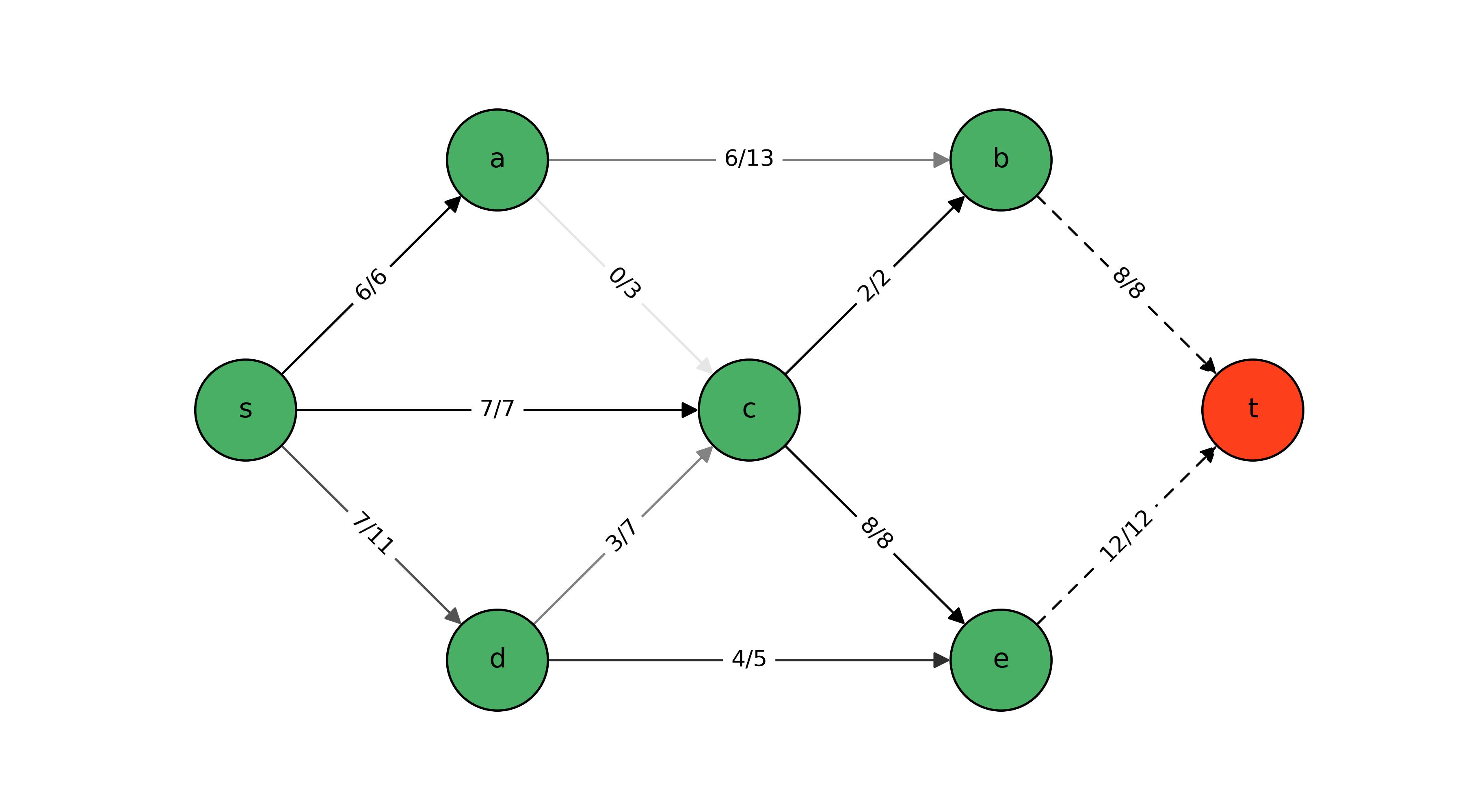
The code for visualizing the solutions by way of solving the Min-Cut problem is much the same. The only differences are that we retrieve the Max-Flow solution values via con_x[i].Pi and the Min-Cut solution values via y[i, j].X and z[i].X. The code and resulting illustration are both shown below.

 1
 2
 3
 4
 5
 6
 7
 8
 9
10
11
12
13
14
15
16
17
18
19
20
21
22
23
24
25
26

fig, ax = plt.subplots(figsize=(9, 5))
ax.set_xlim([-0.25, 4.25])
ax.set_ylim([-0.25, 2.25])

node_size = 2000
edgecolors = 'black'
arrowsize = 15
node_color = ['#49AF64' if z[i].X == z['s'].X else '#FE3F1C'
              for i in V]
style = [(0, (5, 5)) if y[i, j].X == 1 else '-'
         for (i, j) in E]
edge_color = [cm.binary(0.1 + 0.9 * con_x[(i, j)].Pi / c[i, j])
              for (i, j) in E]
edge_labels = {(i, j): '{}/{}'.format(int(con_x[i, j].Pi), c[i, j])
               for (i, j) in E}

nx.draw_networkx(graph, ax=ax, pos=pos, nodelist=V, edgelist=[],
                 node_color=node_color, edgecolors=edgecolors,
                 node_size=node_size)
nx.draw_networkx_edges(graph, ax=ax, pos=pos, edgelist=E,
                       edge_color=edge_color, style=style,
                       node_size=node_size, arrowsize=arrowsize)
nx.draw_networkx_edge_labels(graph, ax=ax, pos=pos,
                             edge_labels=edge_labels)
ax.axis('off')
plt.savefig('mincut-optimal.jpg', dpi=400)

The identified optimal Max-Flow solution again leverages all but edge $(a, c)$; however, a few glances back-and-forth with the previous illustration are enough to see that the Max-Flow solution is subtly different in the bottom part of the graph. Nevertheless, this solution also achieves a flow of 20 from $s$ to $t$. The corresponding optimal Min-Cut solution bipartitions the nodes into ${A=\{s, c, d, e\}}$ and ${B=\{a, b, t\}}.$ It does so by cutting edges $(s, a)$, $(c, b)$, and $(e, t)$ with respective edge capacities of 6, 2, and 12 which again sum to 20.

There are apparently multiple optima for each problem, and Gurobi interestingly identified a different primal-dual pair of optimal solutions when it solved Min-Cut versus when it solved Max-Flow. In solutions identified solving Min-Cut, another implication of complementary slackness is evidenced. Either $x_{ij}^* = 0$ in the Max-Flow problem or ${y_{ij}^* = z_i^* - z_j^* }$ in the Min-Cut problem (or both). So for edge $(i, j)$, if the optimal Min-Cut solution bipartitions the vertices with ${\{j, s\} \subseteq A}$ and ${\{i, t\} \subseteq B}$ , then the corresponding optimal Max-Flow solution has no flow across edge $(i, j)$. This is exhibited by edge $(a, c)$ above.

Wrap Up

In this post, we used gurobipy to solve linear programming implementations of the Max-Flow and Min-Cut problems. For each problem, we were able to construct and visualize a solution to the other by accessing the constraint shadow price (i.e., dual variable) values. By jointly visualizing the Max-Flow and Min-Cut solutions, we were able to observe some implications of complementary slackness conditions that arise as a result of the two problems having a strong dual relationship.