Algebraic modeling languages like JuMP, gurobipy, Pyomo, CVXPY, and PuLP (among others) are widely used for implementing mathematical models. For newcomers, the wide array of available tools may lead to several questions. Which language is best? How do the languages differ? What are their limitations? In this article, I demonstrate the similarity of several modeling languages by presenting example implementations of the Max-Flow problem. The point of this is to show that there is no need to fret – any tool will suffice for getting started with basic modeling. At the end of the article, I distill my experience with modeling languages into a set of bulleted tips for getting started with small projects and and expanding your repertoire to work on larger, more complex projects.

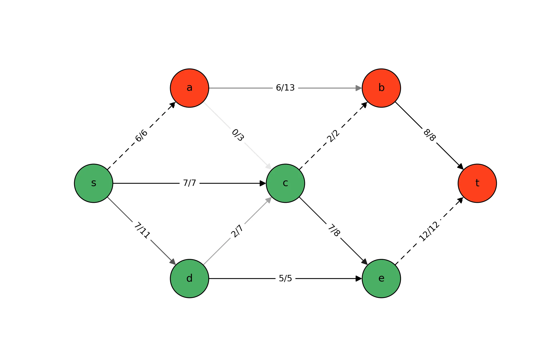
In this post, we leverage the Max-Flow optimization model as an example. For more details about this model, you may refer to my previous posts on the strong primal-dual relationship between Max-Flow and Min-Cut: formulations and implementations. In the former post, we motivate the following linear programming formulation:

Julia

Independent of the modeling tool, the sets and parameters of the Max-Flow problem may be extracted from a mapping of each edge $(i, j)$ to flow capacity $c_{ij}$ using standard Julia programming tools. Below, we show how this may be accomplished by reading that data from a CSV file.

 1
 2
 3
 4
 5
 6
 7
 8
 9
10
11
12
13
14
15
16
17
18
19
20

using DataStructures: DefaultDict

# sets and parameters
E = Vector{Tuple{String, String}}()
c = Dict{Tuple{String, String}, Int64}()
open("limits.csv") do f
    while ! eof(f)
        i, j, cij = split(readline(f), ",")
        push!(E, (String(i), String(j)))
        c[(String(i), String(j))] = parse(Int64, cij)
    end
end
V = collect(Set(Iterators.flatten(keys(c))))
E_hat = cat(E, [("t", "s")], dims=1)
Vp_hat = DefaultDict(Vector{String})
Vm_hat = DefaultDict(Vector{String})
for (i, j) in E_hat
    push!(Vp_hat[i], j)
    push!(Vm_hat[j], i)
end

JuMP

With the sets and parameters already deifned, implementing this problem in JuMP requires only a few more lines of code. Much of the JuMP interface is based on macro invocations (e.g., @JuMP.variable). The purpose of macros is to manipulate existing code or generate new code, a form of metaprogramming.

 1
 2
 3
 4
 5
 6
 7
 8
 9
10
11
12
13
14
15
16
17
18
19
20
21
22
23
24
25
26
27
28
29
30
31

using Printf

import JuMP
import Gurobi

# model
maxflow = JuMP.Model(Gurobi.Optimizer);
JuMP.set_attribute(maxflow, "OutputFlag", 0);

# variables
@JuMP.variable(maxflow, x[E_hat] >= 0);

# constraints
@JuMP.constraint(maxflow, flow_limit[(i, j) in E], x[(i, j)] <= c[(i, j)]);
@JuMP.constraint(
    maxflow,
    flow_balance[i in V],
    sum(x[(i, j)] for j in Vp_hat[i]) == sum(x[(j, i)] for j in Vm_hat[i])
);

# objective
@JuMP.objective(maxflow, Max, x[("t", "s")]);

# solve
JuMP.optimize!(maxflow);

# print solution
@printf("z = %4.1f\n", JuMP.objective_value(maxflow))
for k in E
    @printf("x[%s] = %4.1f\n", k, JuMP.value(x[k]))
end

In the code snippets above, I include comments to indicate where exactly the sets, parameters, variables, constraints, and objective function are defined. As we see in the forthcoming sections, models are all generally implemented in this order regardless of the modeling language. Intuitively, this is because the problems are mathematically formulated in this order. For example, it is impossible to define an indexed variable without first defining the indexing set (both in formulation and implementation).

Python

Again, independent of the specific modeling tool used, the parameters may be defined using standard Python programming tools. This code is designed to precede each of the three Python-based implementations that follow.

 1
 2
 3
 4
 5
 6
 7
 8
 9
10
11
12
13
14
15
16
17
18
19

from collections import defaultdict
from itertools import chain

# sets and parameters
E = list()
c = dict()
with open('limits.csv') as fh:
    for line in fh:
        i, j, cij = line.strip().split(',')
        cij = int(cij)
        E.append((i, j))
        c[i, j] = cij
V = sorted(set(chain.from_iterable(E)))
E_hat = E + [('t', 's')]
Vp_hat = defaultdict(set)
Vm_hat = defaultdict(set)
for (i, j) in E_hat:
    Vp_hat[j].add(i)
    Vm_hat[i].add(j)

gurobipy

A standard way to implement math programming models in gurobipy is via generator expressions. Below, I use this technique to define the flow balance and flow limit constraints. Also, note that gurobipy’s default behavior when declaring variables is to restrict them to the non-negative reals. In all of the other example implementations, we must explicitly declare that the flow variables are non-negative.

 1
 2
 3
 4
 5
 6
 7
 8
 9
10
11
12
13
14
15
16
17
18
19
20
21
22
23
24
25
26
27
28

import gurobipy as grb

# model
maxflow = grb.Model()
maxflow.setParam('OutputFlag', 0)

# variables
x = maxflow.addVars(E_hat)

# constraints
flow_balance = maxflow.addConstrs(
    (sum(x[j, i] for j in Vp_hat[i])\
     == sum(x[i, j] for j in Vm_hat[i]))
    for i in V
)

flow_limit = maxflow.addConstrs(x[i, j] <= c[i, j] for (i, j) in E)

# objective
maxflow.setObjective(x[('t', 's')], grb.GRB.MAXIMIZE)

# solve
maxflow.optimize()

# print solution
print(f'z = {maxflow.getObjective().getValue():4.1f}')
for (i, j) in E:
    print(f'x[{i}, {j}] = {x[i, j].X:4.1f}')

Pyomo

I leverage Pyomo’s decorator syntax to define the constraints and objective as Python functions.

 1
 2
 3
 4
 5
 6
 7
 8
 9
10
11
12
13
14
15
16
17
18
19
20
21
22
23
24
25
26
27
28
29
30
31

import pyomo.environ as penv

# model
maxflow = penv.ConcreteModel()

# variables
maxflow.x = penv.Var(E_hat, domain=penv.NonNegativeReals)

# constraints
@maxflow.Constraint(V)
def flow_balance(maxflow, i):
    return sum(maxflow.x[j, i] for j in Vp_hat[i])\
        == sum(maxflow.x[i, j] for j in Vm_hat[i])

@maxflow.Constraint(E)
def flow_limit(maxflow, i, j):
    return maxflow.x[i, j] <= c[i, j]

# objective
@maxflow.Objective(sense=penv.maximize)
def objective(maxflow):
    return maxflow.x['t', 's']

# solve
solver = penv.SolverFactory('gurobi')
result = solver.solve(maxflow)

# print solution
print(f'z = {maxflow.objective():4.1f}')
for (i, j) in E:
    print(f'x[{i}, {j}] = {maxflow.x[i, j].value:4.1f}')

CVXPY

CVXPY is a Python-based modeling language specifically for formulating convex optimization problems that supports numpy-like syntaxes. Of course, linear programming models are convex, so CVXPY will work for this application. Compared to the other modeling langauges featured in this post, CVXPY differs in that it uses 0-based indexing exclusively to index variables. We circumvent this limitation by defining E_hat_map, a dictionary that maps each edge $(i, j)$ to an integer index. Another minor difference is that CVXPY model instantiation occurs after the variables, constraints, and objective are defined.

 1
 2
 3
 4
 5
 6
 7
 8
 9
10
11
12
13
14
15
16
17
18
19
20
21
22
23
24
25
26
27
28

import cvxpy

# variables
E_hat_map = {(i, j): e for e, (i, j) in enumerate(E_hat)}
x = cvxpy.Variable(len(E_hat), nonneg=True)

# constraints
constraints = list()
for i in V:
    constraints.append(sum(x[E_hat_map[j, i]] for j in Vp_hat[i])\
                       == sum(x[E_hat_map[i, j]] for j in Vm_hat[i]))

for (i, j) in E:
    constraints.append(x[E_hat_map[i, j]] <= c[i, j])

# objective
objective = x[E_hat_map[('t', 's')]]

# model
maxflow = cvxpy.Problem(cvxpy.Maximize(objective), constraints)

# solve
maxflow.solve(cvxpy.GUROBI)

# print solution
print(f'z = {maxflow.value:4.1f}')
for (i, j) in E:
    print(f'x[{i}, {j}] = {x[E_hat_map[i, j]].value:4.1f}')

PuLP

The PuLP implementation is similar in nature to that for gurobipy. The main difference is that the constraints and objective here are added to the model using the addition assignment operator. Under the hood, however, the operator invokes the maxflow.__iadd__ magic method, which is not altogether that different from gurobipy’s maxflow.addConstrs or maxflow.setObjective method invocation.

 1
 2
 3
 4
 5
 6
 7
 8
 9
10
11
12
13
14
15
16
17
18
19
20
21
22
23
24
25
26

import pulp

# model
maxflow = pulp.LpProblem('MaxFlow', pulp.LpMaximize)

# variables
x = pulp.LpVariable.dicts("x", E_hat, cat="NonNegativeReals")

# constraints
for i in V:
    maxflow += pulp.lpSum(x[j, i] for j in Vp_hat[i]) == pulp.lpSum(x[i, j] for j in Vm_hat[i])

for (i, j) in E:
    maxflow += x[i, j] <= c[i, j]

# objective
maxflow += x[('t', 's')]

# solve
solver = pulp.getSolver('GUROBI', msg=0, OutputFlag=0)
result = maxflow.solve(solver=solver)

# print solution
print(f'z = {maxflow.objective.value():4.1f}')
for (i, j) in E:
    print(f'x[{i}, {j}] = {x[i, j].value():4.1f}')

Lessons

Of course, math programming models may be implemented in many other ways using these tools. I chose to present these specific implementations because they are similar in syntax and in style. For small projects, virtually any modeling language will suffice. For tackling larger projects or learning new tools, may advice is as follows.

1. For getting acquainted with math modeling implementations, start with a small project and commit to a single modeling tool. Pick a tool that is compatible with a programming language you feel comfortable using. If you are indecisive, roll a die.
2. Every modeling language ships with examples that showcase its capabilities. Treat those examples as self-guided tutorials. Experiment, tinker, and seek help as needed. In my experience, math modelers are quite friendly!
3. Much of what allows one to be proficient at using a modeling language is first becoming proficient at one of its supported programming languages (e.g., Julia or Python). In my humble opinion, understanding how to massage data into an appropriate format is an undervalued skill, but one that is tremendously useful for efficiently preprocessing and postprocessing model data. Alternate between developing your modeling language and programming language proficiencies.
4. If in the future you find yourself working on a project that demands a feature that is not supported by the modeling tool(s) you know, switch to a modeling tool that possesses that feature. In all likelihood, more than 90% of your already-developed skills are readily transferrable, so you should be able to ramp quickly.
5. Repeat (2), (3), and (4) as necessary.

Let me know if these tips work for you or if you used another approach in the comments. Best wishes to you on your learning and, as always, happy modeling! 🙂